Understanding the Basics of Graph Data Structure

In this post, we will look at understanding the basics of Graph data structure.

Graph is arguably one of the most practically used data structures. For example, below are some of the way graph data structure is useful:

• In the field of computer science, graphs can represent a computational flow.
• Google Maps uses graphs for building their transportation systems. In a map, cities are like vertices and the roads connecting those cities are edges. Basically, graph is an ideal data structure to represent maps.
• If you consider social media, every user is a vertex and their connection are edges. In other words, graphs can describe a social network.
• Also, the whole of internet is a graph. Each page is a vertex and it can link to other pages. Basically, the link is an edge.

There are many other important uses of Graphs. Therefore, it is a very important topic in terms of studying data structures.

1 – What is a Graph Data Structure?

We now know how graphs are useful. Let’s understand how they look like.

Below is an example of a graph.

As you can see, a graph is a collection of nodes. There may or may not be connections between these individual nodes. From a terminology point of view, the nodes are also known as a vertices. In the above example, 0, 1, 2, 3, 4 are the vertices of the graph.

The connections between the nodes are known as edges. For example, the line between nodes 0 and 1 is an edge.

Formally, a graph is a non-linear data structure that consists of vertices connected by edges.

2 – Types of Graphs

While there are many types of graphs, there are a few important ones to know.

They are as follows:

2.1 – Undirected Graphs

These are graphs where the edges do not have any direction property. Below is an example of an undirected graph.

Here, we can move from Node 0 to Node 1. Also, we can move from Node 1 to Node 0 just as easily. In other words, there is no fixed direction in this type of graph.

2.2 – Directed Graphs

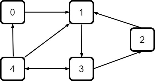
As the name suggests, directed graphs have direction property for their edges. See below example:

As you can see, in the above graph, we can move from Node 0 to Node 1. However, we cannot move from Node 1 to Node 0 directly. We could probably take a longer route to go from Node 1 to Node 3 and then to Node 4 before coming back to Node 0.

2.3 – Weighted Graphs

Another category of graphs is the weighted graph. In this type of graph, the main factor is that each edge of the graph has a fixed weight assigned to it. Weight can also be seen as a cost that has to be paid for traversing a particular edge. In a map, this weight is often the number of kilometres between two cities (or vertices).

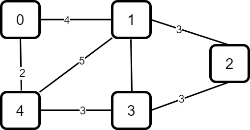
Below is an example of a weighted graph.

As you can see, we represent weights as numbers in the above example. The weight of the edge (or connection) between Node 0 and Node 1 is 4. In other words, 4 units is the cost to be paid while travelling from Node 0 to Node 1.

Weights are often important when trying to calculate shortest path between two nodes in a graph. A practical application could be to find the shortest route between two places on a map.

2.4 – Unweighted Graphs

As the name suggests, this is basically the opposite of weighted graphs. In other words, there is no explicit cost attached to an edge in a weighted graph.

Below is an example:

All edges have equal cost in the above graph.

Another important thing to consider is that these types are not always standalone. For example, a graph can be directed and weighted. It can also be directed and unweighted. Similarly, an unweighted graph can also be undirected as in the above example.

3 – Representation of Graph Data Structure

The next important aspect to consider in understanding graph data structure is how to represent a graph.

There are two major ways in which we can represent graphs.

3.1- The Adjacency List

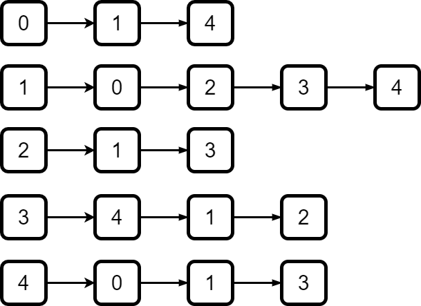
In an adjacency list, we use an array of lists to represent a graph. The size of the array is equal to the number of vertices.

For the graph in the examples above, below is how the adjacency list would look like.

To understand it better, let’s take the example of Node 0. In the graph, it connects to Node 1 and Node 4. The same is represented in the adjacency list.

Node 1 connects to Node 0, 2, 3 as well as 4. Hence, we represent it as such in the list.

Note that the list can be a linked-list or even an array.

The main advantage of adjacency list is that it saves a lot of space while representing a graph especially if the graph is sparse. In other words, if a graph has lot of nodes that don’t connect with many other nodes, then adjacency list is ideal. Also, insertion and deletion of nodes to a vertex is easier with adjacency lists.

On the downside, adjacency lists can be slow.

3.2 – The Adjacency Matrix

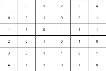
The second way of representing a graph is to use an adjacency matrix. In this representation, we basically construct a n * n size matrix.

So, if there are 5 vertices in our graph, we will have a matrix of 5 * 5 size. If we have hundred vertices, we get a matrix of 100 * 100.

Below is same graph representation in adjacency matrix format:

The matrix itself is quite self-understandable. For example, for Node 0 only Node 1 and Node 4 have true as the entry meaning that there is an edge between those vertices. For the other nodes, we mark the flag as 0 to signify no connections.

Similarly, the matrix is described for other nodes as well.

The advantage with adjacency matrix is that it is easier to follow. Also, implementation is easy.

However, on the downside, an adjacency matrix consumes a lot more memory.

Conclusion

With this, we have successfully built an understanding on the basics of graph data structure. We also looked at various types of graphs and also the different ways of representing a graph data structure.

In the next post, we will implement the graph data structure.